What is a confidence interval? I wanted to know that recently and turned to one of my favourite books: Measuring the User Experience, by Tom Tullis and Bill Albert. And here’s what they say:
“Confidence intervals are extremely valuable for any usability professional. A confidence interval is a range that estimates the true population value for a statistic.”
Then they go on to explain how you calculate a confidence interval in Excel. Which is fine, but I have to admit that I wasn’t entirely sure that once I’d calculated it, I really knew what I’d done or what it meant. So I trawled through various statistics books to gain a better understanding of confidence intervals, and this column is the result.
Our starting point is the need for a measurement
But sooner or later, we’ll have to tangle with some quantitative data. Let’s say, for example, that we have this goal for a new product: On average, we want users to be able to do a key task within 60 seconds. We’ve fixed all the show-stoppers and tested with eight participants—all of whom can do the task. Yay! But have we met the goal? Assuming we remembered to record the time it took each participant to complete the task, we might have data that looks like this:
|
Participant
|
Time to Complete Task (in seconds)
|
|---|---|
|
A |
40 |
|
B |
75 |
|
C |
98 |
|
D |
40 |
|
E |
84 |
|
F |
10 |
|
F |
33 |
|
H |
52 |
To get the arithmetic average—which statisticians call the mean—you add up all the times and divide by the number of participants. Or use the AVERAGE formula in Excel. Either way, the average time for these participants was 54.0 seconds. Figure 1 shows the same data with the average as a straight line in red.

Well, maybe. If our product has only eight users, then we’ve tested with all of them, and yes, we’re done. But what if we’re aiming at everyone? Or, let’s say we’re being more precise, and we’ve defined our target market as follows: English-speaking Internet users in the US, Canada, and UK. Would the data from eight test participants be enough to represent the experience of all users?
How does ‘true population value’ compare to our sample?
Our challenge, therefore, is to work out whether we can consider the average we’ve calculated from our sample as representative of our target audience.
Or to put that into Tullis and Albert’s terms: in this case, our average is the statistic, and we want to use that data to estimate the true population value – that is, the average we would get if we got everyone in our target audience to try the task for us.
One way to improve our estimate would be to run more usability tests. So let’s test with eight more participants, giving us the following data:
|
Participant
|
Time to Complete Task (in seconds)
|
|---|---|
|
I |
130 |
|
J |
61 |
|
K |
5 |
|
L |
53 |
|
M |
126 |
|
N |
58 |
|
O |
117 |
|
P |
15 |
Then, we can calculate a new mean.
Oh, dear… For this sample, the arithmetic average comes out to 74.6 seconds, so we’ve blown our target. Perhaps we need to run more tests or do more work on the product design. Or is there a quicker way?
Arithmetic averages have a bit of magic: the Central Limit Theorem
Luckily for us, means have a bit of magic: a special mathematical property that may get us out of taking the obvious, but expensive course – running a lot more usability tests.
That bit of magic is the Central Limit Theorem, which says: if you take a bunch of samples, then calculate the mean of each sample, most of the sample means cluster close to the true population mean.
Let’s see how this might work for our time-on-task problem. Figure 2 shows data from 10 samples: the two we’ve just been discussing, plus eight more. Nine of these samples met the 60-second target, one did not. The data varies about from 10 to 130 seconds, but the means are in a much narrower range.

The chance that any individual mean is way off from the true population mean is quite small. In fact, the Central Limit Theorem also says that means are normally distributed, as in the bell-curve normal distribution shown in Figure 3.

- Two things define them:
- where the peak is – that is, the mean, which is also the most likely value
- how spread out the values are – which the standard deviation – also known as sigma – defines
- The probability of getting any particular value depends on only these two parameters – the mean and the standard deviation.
Figure 4 shows two normal distributions. The one on the left has a smaller mean and standard deviation than the one on the right.

We can use the Central Limit Theorem to find a confidence interval
If you’re still with me, let’s get back to our challenge: deciding whether our original mean of 54.0 seconds from the first eight participants was sufficiently convincing to show that we’d met our target of an average time on task of less than 60 seconds and would allow us to launch. We’d rather not run nine more rounds of usability tests; instead, we want to estimate the true population mean.
Fortunately, the Central Limit Theorem lets us do that. Any mean from a random sample is likely to be quite close to the true population mean, and a normal distribution models the chance that it might be different from the true population mean. Some values of the true population mean would make it very likely that I’d get this sample mean, while other values would make it very unlikely. The likely values represent the confidence interval, which is the range of values for the true population mean that could plausibly give me my observed value.
To do the calculation, the first thing to decide is what we’re prepared to accept as likely. In other words, how much risk are we willing to run of being wrong? If we’re aiming for a level of risk that is often stated as statistical significance at p < 0.05, the risk is a 5% chance of being wrong, or one in 20, but there is a 95% chance of being right.
The next thing we need is a standard deviation. The only one we have is the standard deviation of our sample, which is 29.40 seconds. (I used Excel’s STDEV.S command to work that out.)
Finally, we plug in the mean, which is 54.0 seconds, and the number of participants, which is 8.
You can work this out with formulas and a calculator, but let’s use Excel. The CONFIDENCE command does it, giving us a value that we can
- subtract from the sample mean to get the lowest true population mean that our observed mean could plausibly have come from
- add to the sample mean to get the highest true population mean that our observed value could plausibly have come from
The result: the 95% confidence interval for the mean is 29.4 to 78.6 seconds, in comparison to our target of 60 seconds.
This is unfortunate. If the true population mean were as high as 78.6 seconds, we could still have obtained our sample mean of 49.4 seconds with a 95% probability. Oh, dear. That would be 18.6 seconds greater than our task-time target, which is disappointing all around. But we wouldn’t be nearly as worried if the true population mean happened to fall at the low end of the range. That would mean we’ve met our target.
Confidence intervals aren’t always correct
Remember that 95%, which says that about one time in 20 you’re likely to get it wrong? You wouldn’t know whether this time is the one time in 20. If that makes you feel uncomfortable, you’ll need to increase your confidence level, which will also increase the range of the confidence interval, so you’ll have a greater chance of catching the true population value within it.
Here are the confidence intervals for this sample, for some typical levels of risk:
|
Confidence Interval (in seconds)
|
|||
|---|---|---|---|
|
Risk of Being Wrong
|
Confidence Level
|
Lower End
|
Upper End
|
|
20% |
80% |
39.3 |
68.7 |
|
10% |
90% |
34.3 |
73.7 |
|
5% |
95% |
29.4 |
78.6 |
|
1% |
99% |
17.6 |
90.4 |
You can see that, as we reduce the risk, we increase the confidence level and end up with a wider confidence interval – and in this example, also have an increasing level of depression about that launch date.
Have you come across Six Sigma, the quality improvement program that Motorola originated, which is now popular in many manufacturing companies? They wanted to be very, very sure that they knew the risk of manufacturing poor-quality products and chose a confidence level of 99.99966% – that is, 3.4 chances in a million. I didn’t bother calculating the confidence interval for our sample to get a Six-Sigma level of risk, because it would constitute the whole range of our data.
Confidence intervals depend on sample size
What do you do if you want to get a higher confidence level, but also need to be sure you’ve met your target for the mean? Increase the sample size.
The more data in your sample, the smaller your confidence interval. That’s because with more data, you have more chance of the sample being a pretty good match to the whole population and, therefore, of its mean being similar to the true population value.
In my example, I’ve got 80 participants overall. The mean for all of the participants is 47.1 seconds, and the 95% confidence interval is (39.8, 54.4). So if I’d tested with a lot more people, I would indeed have proven that we’re okay to launch, because the highest plausible value is less than my target of 60 seconds.
That’s part of the fun of confidence intervals: we want to calculate a confidence interval so we don’t have to do as much sampling, but to get a narrow confidence interval, we need to do more sampling.
The Central Limit Theorem works only on random samples
I recently read an article on sample sizes that asserted, “One thousand sessions provide a sufficiently narrow margin of error (plus or minus 2.5% at a 90% confidence level).”
This is true, but only if the sample is a random sample. For example, let’s say we wanted the average time it took to complete the New York Marathon across 45,000 runners. If we took a random sample of just 1000 runners, we would get a narrow confidence interval. But if we took the times of the first 1000 runners across the finish line, we’d get something very far indeed from the true population mean.
The mean is convenient, but not always helpful
So far, I’ve used the example of a target for a mean value: The average time on task must be less than a specified target.But would that be a good target to have?
Figure 5 shows a set of data that is quite typical for user experience: a peak at low values – for example, task times – then a long tail with a few values that are much higher. It’s the overall data set that our samples have so far come from. The mean is 50.3 seconds, which is lower than the target of 60 seconds.
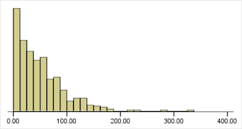
Also, look at the way most of the values pile up at the shorter end. Those users ought to be happy – the time it took them to complete the task is much shorter than the advertised time. But to ensure that a high volume of users can achieve those task times once the system gets rolled out, we’ll have to make sure that the system can cope with that high peak of very fast task times. So our colleagues who are managing system performance are likely to be far more interested in the most frequent value, which is the mode, than in the mean. But you can’t calculate a confidence interval for the mode either.
Of course, Excel can take any numbers you put in and shove them through the calculation – so if you mistakenly try to run a CONFIDENCE formula on a mode, you’ll get an output. But it won’t be meaningful, because there is no Central Limit Theorem or any equivalent for modes.
Summary: confidence intervals can save you effort
The confidence interval for the mean helps you to estimate the true population mean and lets you avoid the additional effort that gathering a lot of extra data would require. You can compare the confidence interval you calculated with the target you were aiming for.
Once you have worked out what level of risk you are willing to accept, confidence intervals for the mean are easy to calculate. You’ll need these formulas in Excel:
- AVERAGE – to get the mean of your sample
- STDEV.S, in Excel 2010, or STDEV, in earlier versions – to get the standard deviation of your sample
- CONFIDENCE – to calculate the amount to subtract from the mean to get the lower end of the confidence interval and to add to the mean to get the upper end.
Acknowledgement: Confidence image by Sandwich, creative commons
#surveys #surveysthatwork